Create A Simple 3-Generation Family Tree In Excel (Tutorial)

This tutorial takes you step-by-step through creating a simple three-generation family tree in Microsoft Excel.

This type of tree is a great project for school or as a gift from children to grandparents.

Our tips and tricks will help you avoid fiddling endlessly with dragging lines and positioning pictures in Excel.

If you want more generations, we have separate tutorials for

Table of Contents

What A Simple Family Tree Looks Like

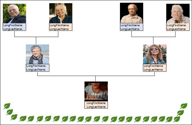
Before we get started, you should understand the end result. The simple family tree prints in landscape mode like this:

Video Walkthrough

If you prefer a video walking through these steps, here you go.

Step 1: Create A Blank Worksheet With A Landscape Print Area

We want to create a tree that prints on a single A4 sheet in landscape mode.

So, it’s important to see where the boundaries are when we’re adding elements to the worksheet.

The first thing to do is to show those boundaries while you’re working. That means you won’t step outside them.

Click on the File menu and choose the Print menu item. You’ll see that the default print mode is Portrait, which isn’t what we want.

Toggle the setting to Landscape mode and click the back arrow (top left).

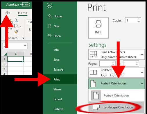
You will now see dashed lines on your blank spreadsheet that mark the boundaries.

If you’re working on a small screen, you may need to scroll right or down a bit to see the lines.

Step 2: Set The Font And Column Widths

The default font in the latest versions of Excel is Calibri, which I’m not fond of.

I change the font to Arial and size 11. To do so:

Select the entire spreadsheet (ctrl-A).
Use the Home ribbon to change the font and size.

I promised you tips so you don’t have to fiddle and experiment with column widths.

You are going to work with seven columns: A to G.

Select columns A to G
Right-click and choose “Column Width” from the drop-down menu.
Change the width size to 16.5.

You should now double-check that columns A to G still fit within the landscape print area.

If you notice that column G is past the print area, you are probably using a different font or character size than I do.

That’s okay. But be sure to decrease the column widths slightly to ensure that the fourth grandparent fits on the page.

Step 3: Create The Name Area For The First Grandparent

My preference is to have first names and last names on two lines. This allows space for very long names.

I place a photo of the grandparent above the name. You may want to have it below the name, but I suggest you follow my instructions to the end. Then you can tinker with the layout.

For grandparents, the first name is on Row 7 and the last name is on Row 8.

Enter the paternal grandfather’s first name into cell A7 and last name into A8.
Set the background color of these two cells to light blue.

We’ll leave the photos until later. We haven’t finished formatting the text display for grandparent number one.

Step 4: Ensure That Names Don’t Overflow

This step is optional if the first and last names in your family tree are not exceptionally long.

We want to ensure that a long name doesn’t spill into the next cell. The display should truncate the name to the width that we specified.

In other words, the surname “Wigglesworthingtonblessett” will display as “Wigglesworthingt”.

You’ll find several “how-to” instructions online on how to do this. I find that several of these methods don’t always work.

This one method is the one that works for me: add a space into the cell next door!

In other words, click into cells B7 and B8 and enter a space.

Step 5: Put A Border Around The Name Fields For Grandpa #1

You probably know that although your new spreadsheet is showing gridlines, they don’t show on the printed page.

But we want the names to appear within a single box. You don’t have to merge the cells to achieve this. Follow these simple steps:

Select cells A7 and A8.
Right-click and choose “Format Cells” from the drop-down menu.
Choose the Border tab.
Choose the “Outline” preset border.

Step 6: Create Three More Grandparent Areas

Instead of repeating the above actions, we’ll simply copy the four formatted cells to create the other areas in this generation.

When I say four cells, I mean the two colored name cells and the two cells to their right.

Then we’ll apply some extra editing.

Select cells A7, B7, A8, and B8 and copy them (ctrl-c)
Click into cell C7 and paste the four cells (ctrl-v)
Repeat into cells E7 and G7

Grandpa #1 is now named in every position! Edit the names of the three grandparents to be correct.

Or blank out the names if you’re preparing this for a younger person to fill in.

We set the color of Grandpa to a light blue, but it’s traditional to have a lighter color for women. This is just a visual cue and is certainly not mandatory!

But for a contrasting look, you can change the background color of the two grandmothers to light pink.

Step 7: Create the Two Parent Areas

We now move down a generation.

We want the name cells to be similarly formatted, so you can use Grandpa #1 again as the template.

Select cells A7, B7, A8, and B8 and copy them (ctrl-c).
Click into cell B18 and paste the four cells (ctrl-v).
Repeat into cell F18.

The last thing to do here is:

Change the background color of the mother entry.
Edit both names to be correct.

Step 8: Create The “Home” Person

This is the lowest entry in the tree.

Select cells A7, B7, A8, and B8 and copy them (ctrl-c).
Click into cell D29 and paste the four cells (ctrl-v).

Edit the background color and name accordingly.

We now have the names spaced out in the correct layout. The next steps are to add the traditional connecting lines in a family tree.

About Creating Connecting Lines In Excel

The goal is to achieve this look:

Because Excel isn’t a graphics tool, this isn’t as easy it should be. Part of the challenge is to overcome the finicky nature of drawing lines in Excel. We’ve got some handy tips for you.

Quick tip: draw lines before adding images

I recommend that you draw full lines before adding photographs or flags. Any images added after the lines will plonk on top of them.

Let’s say you take the opposite approach and add the images first, and then add lines to the edge of the image.

The problem is that if you later want to remove the images, your lines will be too short and will need further editing.

Step 9: Create The First Short Vertical Line Under Grandpa #1

Create the first short vertical line on the left of the diagram with these steps:

Go to the “Insert” tab in the top ribbon.
Expand the “Illustrations” drop-down.
Expand the “Shapes” option.
Choose the line without arrows.

Place your cursor below the box for Grandpa 1, somewhere near the middle of column A. Drag the cursor down to create the line.

Don’t worry about the placement or height, you just want to create a short straight vertical line in the general area.

Now you have the line, we’ll format it correctly.

The default line is probably a light blue color. I prefer to change this to black.

Right-click the line and choose “Format Shape”.
Edit the “Color” to black.

Set the height to 1 cm

The next step is to set the height (length) of the vertical line to 1 cm.

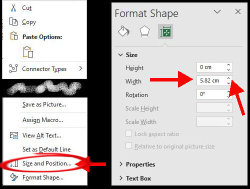
I recommend that you don’t use the cursor to drag lines to an unknown height. Instead, use the precise height control with these steps:

Right-click the line and choose “Format Shape”.
Switch to the “Size and Properties” tab.
Edith the Height to 1 cm.

Position the line correctly

The final step here is to position the line halfway along the bottom of the last name cell.

My tip is to edit the last name for Grandpa #1 to random letters that fill the entire cell. You can enter “Verylonglastname” for example.

Depending on the font you’ve chosen, there will be 13-16 characters displayed. You just need to position the line under the middle letter.

With our example, the line should be under the “g”. This isn’t exactly half with scientific precision, but it’s close enough for the human eye.

Tip: use the positioning circle

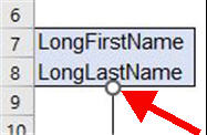
To position the line, drag it to intersect with the bottom of the last name cell.

When you drag and drop the line, you will see a small circle at the top and bottom of the line. You can use the circle to position the end of the line to intersect with the name box.

If you’re used to fancier graphic software, you may expect the line to snap into place. It doesn’t.

You may find that you’ve pushed it up too far so that the line runs into the name box. Here’s our next tip.

Tip: use arrow keys for precise positioning

If you’re as clumsy as me, then positioning the line can get frustrating. Here’s my best tip: don’t use the mouse. Instead, use the arrows on your keyboard.

When the line is selected, a click on an arrow nudges the line slightly in the right direction.

Watch the circle as you nudge the arrow up or down. Click away to see whether you’ve hit the exact spot.

Tip: ensure the line is straight

When you drag lines in Excel, it’s easy to be left with a slight angle i.e. it’s not exactly vertical or horizontal.

You might think the “Rotation” property in the Size control lets you control this. But it doesn’t.

There may be some trick to using the shape properties to get a zero-degree angle, but I haven’t found it.

Instead, click the edge of the line and use the cross-hairs to judge when the angle is zero.

Excel and younger folk

This may all be too finicky for small people with school projects.

I suggest you place the arrows for them and leave them with the fun of adding decorative images to the tree (final steps).

Step 10: Create The Second Vertical Line Under Grandma #1

You’ll be happy to hear that this step is only a copy-and-paste job.

We want a line of the same height, color, and position under Grandma #1.

To avoid going through the positioning steps again, don’t copy the actual line under Grandpa #1.

Instead, copy the cells that contain the line!

In this case, it will be cells A9 and A10. Just highlight both cells and copy them to cells C9 and C10.

The line is positioned exactly where you want it. Hurrah!

Step 11: Create The First Horizontal Line Between Grandparents

Repeat the instructions in Step 10 to insert a line, but this time place it so that it is horizontal.

Again, don’t worry about the length or position at this point. But change the color to be black.

Drag the horizontal line so that the left edge intersects with the bottom of the vertical line under Grandpa #1.

You may not be able to position it exactly through drag-and-drop (I can’t). So, drop to as close as you can and use the arrow keys to nudge it into place.

Once you have the left edge anchored, you can adjust the length.

My tip is to use the height control instead of drag-and-drop. It’s far easier to fine-tune.

Right-click the horizontal line and choose “Format Shape”.
Switch to the “Size and Properties” tab.
Use the “up” arrow in the Width control to nudge the length to the right.

Step 12: Create The Long Vertical Line From Grandparents To Father

This time, you want to position the line at the middle of column B.

Again, my advice is to edit the father’s first name to fill the cell. Then use the middle letter as your guide.

I won’t repeat the exact steps for positioning. But I advise that you follow this sequence for the easiest experience.

Start with a short black vertical line that meets the father’s box.
Use the up arrow to nudge the short line up to meet the long horizontal line.
Open the shapes property and use the height control to lengthen the arrow back down to meet the father’s name box.

Step 13: Copy The Intersecting Lines To The Maternal Grandparents

You’ll be glad to hear that you can simply copy the cells without change to make the lines for the second pair of grandparents.

Highlight the cells from A9 to C17.

Place your cursor in cell E9 and paste all the cells. That’s it for this generation!

Step 14: Create The Intersecting Lines For Parents And Child

We’ll start by copying the lines from the paternal grandparents and then we’ll edit the positioning.

Highlight the cells from A9 to C17.
Place your cursor in cell B20 and paste all the cells.

You now have the correct number of lines, but they aren’t aligned correctly.

Use the right arrow to move the right-most vertical line to the center of column F.
Use the width property to widen the horizontal line to intersect with it.

And that’s it!

You now have the simple 3-generation family tree structure in Excel.

You can stop now and work with what you’ve got i.e. add the correct names and print out the sheet.

But if you want some photos in there, let’s keep going.

Preparing Photos For Your Simple Tree

In our example tree, we have cropped images with faces.

Because the spreadsheet images must be small, you probably have some preparation and editing to do to get similar images from your family photos.

My advice is to prepare images in either of these size units:

90 X 90 pixels
2.38 cm X 2.38 cm

If you don’t have a favorite editing app for cropping and sizing photos, I recommend the free version of Canva.

You just need to register an email at Canva.com.

Step 15: Add Images To The Tree

I’ve left plenty of space for an image above each name box.

You will likely have to make small adjustments to the size of your image once you’ve pasted it. Repeat these steps for each image:

Put your cursor a few cells above the appropriate name box.
Go to the Insert tab in the ribbon.
Expand the Illustrations drop-down and choose “Pictures”.
Choose “from This Device”.
Find the correct image on your machine.

Excel plonks the image onto the spreadsheet. You can now adjust the position.

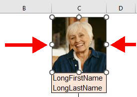
The name cells are about 16 pixels wide. Your images may be slightly wider or narrower. To be visually pleasing, you probably want them centered relative to the name cell.

I recommend that you use the arrow keys to align the image to sit on top of the name box.

Again, use the arrow keys to nudge the image left and right.

You can also widen or narrow the images within Excel by using the handles on the picture object containing the image.

There’s no harm in a little adjustment, but you don’t want to distort a face too much.

Adjusting For Minor Image Differences With The Printed Version

As you work with positioning your pictures in Excel, you’ll probably notice that there can be tiny discrepancies between how the layout looks in the spreadsheet versus how it looks when printed.

I find that images that seem aligned perfectly with the name box are slightly to the left or right in the printed material.

When the bottom of the image seems perfectly adjacent to the top of the name box, the printed version has a tiny gap.

That may not bother you. But if you’re like me, you’ll want the print-out to look perfect.

Thankfully, the Print Preview is accurate to what is printed. You’ll see the discrepancies there, without having to use up your ink.

The trick is to toggle back and forth to the Print Preview while making tiny adjustments to the spreadsheet.

I found that with some images, I had to nudge them down so they seem to be overlapping the name box. But they print perfectly (without a gap, but no overlap).

With other images, I had to shift them slightly to the right or left so that they were misaligned in the spreadsheet view. But they were perfectly aligned in the Print Preview and printed version.

It’s a bit of trial and error. But with only three generations, it shouldn’t take too long.

Getting Creative

In the opening picture in this article, I showed a sample family tree with some extra leafy imagery at the bottom.

I simply used the free stock images and icons that come with Microsoft Excel. You can browse through the collection via the Illustrations drop-down menu.

Get Our Done-For-You Bundle

Does this all seem like too much fiddling around? I’ve prepared a bundle of four formatted templates:

the classic family tree with name boxes
a template formatted for added photos
a template formatted for location flags
a template formatted for photos and flags

In addition, I’ve included perfectly-sized images for 50 U.S. state flags and 48 country flags.

All this for the price of a cup of coffee. Grab it at our Gumroad store here: