Create An 8-Generation Pedigree Family Tree In Excel (Tutorial)

An eight-generation family tree goes back to 128 great-great-great-great-great-grandparents.

This tutorial shows you how to create one in Microsoft Excel that prints across four portrait pages.

The printed pages can be easily taped together to put up on a wall as a single display.

If you’re too busy for the eighteen steps in this tutorial, jump down to the end to grab our “done for you” Excel template bundle.

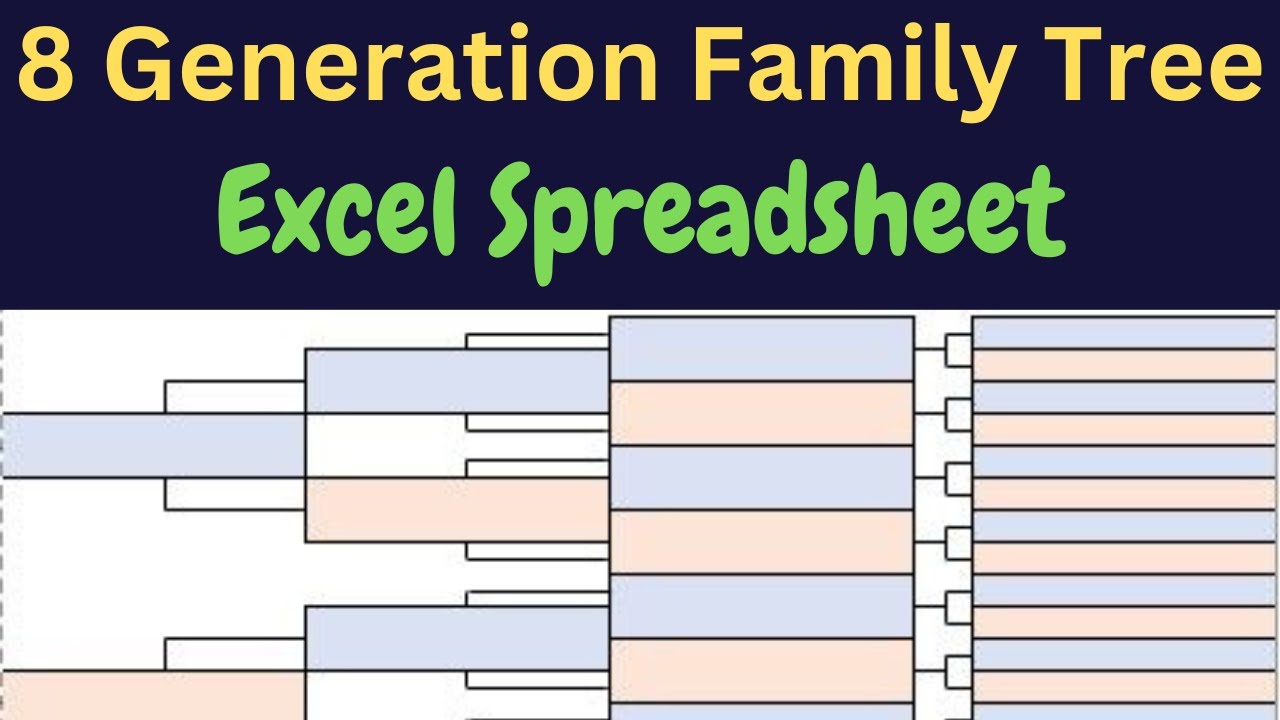
What An 8-Generation Pedigree Tree Looks Like

The picture below is what the top two pages look like in portrait mode in Excel. This is your paternal half of the tree.

Of course, you don’t need to include photos in your tree.

I’ve marked the page boundary with an arrow. You can tape the two printed pages to have a single display.

I’m not showing the bottom two pages – that is the maternal half of the tree. It looks very similar!

Want a tree that fits on one printed page?

It just can’t be done with an eight-generation tree. Trust me, I’ve tried!

But you can do it with seven generations or less. Check out these tutorials:

• seven-generation tree on one Excel page
• six-generation tree on one Excel page
• five-generation tree on one Excel page

Want a bigger tree?

Here you go:

• create a nine-generation tree in Excel
• create a ten-generation tree in Excel

Video Walkthrough

If you prefer a video walkthrough, here you go (click on the play button):

Step 1: Create A Blank Worksheet That Prints In Portrait Mode

New spreadsheets print in portrait mode by default.

So all you have to do here is create a new worksheet.

Step 2: Set The Column Widths

We are going to work with columns A to J.

To change the width of any column, follow these steps:

1. Select the entire column by clicking on the letter at the top.
2. Right-click and choose “Column Width” from the drop-down menu.
3. Enter a size.

Set these sizes:

• Set column A to size 1.
• Set columns B to H (seven columns) to size 19.
• Set column I to size 3.
• Set column J to size 19.

Step 3: Set The Row Heights

We will work with rows 1 to 134.

To fit eight generations onto the page, we need at least 128 rows – one for each 6^th great-grandparent.

The default row height in Excel only fits 33 rows. Obviously, we need to reduce the row height. The challenge is to be sure that the text is still legible.

I find that a row height of 11.5 is the best size.

1. Select the entire sheet using ctrl-A.
2. Right-click anywhere on the sheet.
3. Choose “Row Height” from the menu.
4. Enter 11.5 as the height.

Step 4: Start With The Father Name Field

We are going to fill out the paternal half of our 8-generation tree.

Then we can save a huge amount of time by copying this to the maternal half.

Follow these steps to create the field for the father.

Merge two sets of cells

1. Select cells C35 and C36.
2. Right-click and choose “Format cells”.
3. Switch to the Alignment tab.
4. Check the “Merge cells” box.

Add an outside border

Place a border around cells C35 and C36 with these steps:

1. Right-click and choose “Format Cells” from the drop-down menu.
2. Choose the Border tab.
3. Choose the “Outline” preset border.

Set the font type and size of the merged cells

In order to fit names into this small row height, we need to set the font size to 8.

But the default font of Calibri or Arial doesn’t look great at small sizes. I find that Segoe UI displays and prints well at that size.

1. Select the merged cells.
2. Go to the Home tab in the top menu ribbon.
3. Change the font type to “Segoe UI”.
4. Set the font size to 8.

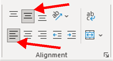
Set the text alignment

I prefer names to be left-justified and vertically centered in the merged cells.

1. Select the merged cells.
2. Set the vertical alignment to Middle Align.
3. Set the horizontal alignment to Left.

Here is a picture of these alignment choices:

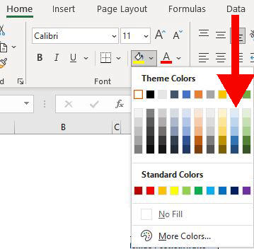
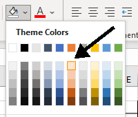
Format the coloring

I like to use a different color in the name field for male and female ancestors.

My preference is a light blue for males.

To change the color of the name field:

1. Select the merged cells.
2. Set the background color to light blue.

Step 6: Copy For Male Ancestors From The 3^rd To 7^th Generations

We are going to use copy-and-paste as much as possible in this process!

I’ve already worked out where each ancestor should go. You’re welcome.

Select and copy the two cells C35 and C36.

Select each cell below in turn and paste the selected range into the cell. This copies the two cells.

3^rd Generation

• D19

4^th Generation

• E11
• E43

5^th Generation

• F7
• F23
• F39
• F55

6^th Generation

• G5
• G13
• G21
• G29
• G37
• G45
• G53
• G61

7^th Generation

• H4
• H8
• H12
• H16
• H20
• H24
• H28
• H32
• H36
• H40
• H44
• H48
• H52
• H56
• H60
• H64

We’ll deal with the eighth generation later.

Step 7: Create The Paternal Grandmother

This is the first female box on the page.

The steps are the same as for the father, except for the position and background color.

Select and copy the two merged cells C35 and C36.

Paste into cell D51.

Change the background color to light orange.

Step 8: Copy For Maternal Ancestors In The 4^th To 7th Generations

Select and copy the merged cells D51 and D52.

Paste the range into the cells listed below. This copies the two merged cells.

4^th Generation

• E27
• E59

5^th Generation

• F15
• F31
• F47
• F63

 6^th Generation

• G9
• G17
• G25
• G33
• G41
• G49
• G57
• G65

7^th Generation

• H6
• H10
• H14
• H18
• H22
• H26
• H30
• H34
• H38
• H42
• H46
• H50
• H54
• H58
• H62
• H66

We’ll deal with the 8^th generation next.

Step 9: Create The 8^th Generation

This furthest generation has a different format from the others.

 In order to fit the 128 people onto two portrait pages deep, I can only give a single row to each.

That means that the display looks a little squeezed for this generation. But it’s still clearly legible.

We’ll format the first male and female boxes. Then we can copy them down the column.

1. Set the color of cell J4 to light blue.
2. Put an outside border around J4.
3. Set the color of cell J5 to light orange.
4. Put an outside border around J5.

Now copy these two cells down as far as J67 is filled with a pink cell.

Ensuring truncation

We have one problem with the cells of column J. Unlike the other ancestor boxes, these cells aren’t merged.

That means that longer names that have more characters than fit in the cell will spill over into the adjacent cell. They will not truncate.

The simplest way to ensure truncation is to put a space into the adjacent cell i.e. in column K.

1. Enter a space into cell K4.
2. Copy K4 all the way down to K67.

And that’s it! We’ve got the paternal half of our ancestor fields.

Now we’ll create the connector lines for this half of the tree.

Adding, Positioning, And Sizing Lines In Excel

If you haven’t worked with lines in Excel, here is how to add one to the sheet:

1. Go to the “Insert” tab in the top ribbon.
2. Expand the “Illustrations” drop-down.
3. Expand the “Shapes” option.
4. Choose the line without arrows.
5. Place your cursor into a cell roughly in the area of where you want it.
6. Drag the cursor horizontally or vertically to create a line.

Changing the color to black

1. Right-click the line and choose “Format Shape”.
2. Change the color from blue to black.

Changing the length of the line

I recommend that you don’t lengthen or shorten lines by dragging the edges. It’s very finicky to get right.

Instead, I’ll give you the exact dimensions to enter into the height and width controls.

1. Right-click the line and choose “Format Shape”.
2. Switch to the “Size and Properties” tab.
3. Use the height property to edit the length of vertical lines.
4. Use the width property to edit the length of horizontal lines.

You can use the arrows to increase or decrease the size.

If you need to enter a size like “2.5 cm”, then you can input it directly into the box.

Use arrows for precise positioning

Once you’ve added the line anywhere on the sheet, you can drag it into the general area where it should be.

You can then use the arrow keys on your keyboard to nudge the lines into the precise position.

Step 10: Create The Connector Lines From The Father To His Parents

The configuration looks like this:

The vertical lines above and below the name box are sized at 5.9 cm.

Two short horizontal lines connect the ends to the edge of the parent boxes. The horizontal lines are sized 1.5 cm.

Step 11: Create The Connector Lines From The 3^rd To 4th Generations

There are two sets of connector lines involved here but you just need to position the first set.

I’ll give you a great tip for copying them down to the other ancestors of this generation.

Create and position the vertical and horizontal line above the blue grandfather box as shown in the picture below:

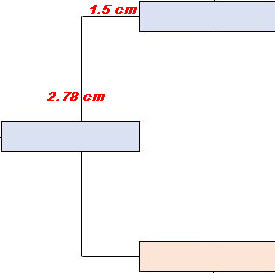
The vertical line is 2.78 cm and the horizontal line is 1.5 cm.

Repeat to position a vertical and horizontal line below the blue grandfather box.

Fast-Copy For the Other Ancestors In This Generation

You’ll be pleased to hear that you don’t have to copy individual lines to finish out this generation’s connector lines.

Instead of copying lines, we simply copy the range of cells that surround the lines. That’s much easier.

1. Select and copy the cell range from D11 to D18.
2. Paste into cell D43.
3. Select and copy the cell range from D21 to D28.
4. Paste into cell D53.

That’s it for this generation.

Step 12: Create The Connector Lines From The 4th To 7th Generations

You now know how to position and copy lines.

So, I’m going to focus on the heights and widths.

All the horizontal lines are 1.7 cm long.

The vertical lines differ by generation:

• 4^th generation: 1.16 cm
• 5^th generation: 0.4 cm
• 6^th generation: 0.2 cm

Step 13: Create The Connector Lines From The 7^th To 8^th Generation

This can be either very simple or a bit tricky. Here are two options:

Easier option

If you want to take the simple route, use a single horizontal line that connects the child and parent like in this picture:

Copy and resize a horizontal line to 0.37cm for this option.

Position it along the bottom gridline of cell I4.

Then copy cell I4 and paste it into all the cells in this column down to I67.

Trickier option

I prefer the fork to look like in this picture:

The challenge is that the four lines are very small and a bit finicky to move into position.

The left horizontal line (the handle of the fork) is 0.4 cm.

The two horizontal lines (the tines of the fork) are 0.3 cm.

The vertical line is 0.4 cm.

Once you have them positioned in the fork structure in cells I4 and I5, copy and paste the cells all the way down to I66 and I67.

Step 15: Create The Maternal Half Of The Tree

Thankfully, we’re not going to repeat the steps for the paternal half. We’re simply going to copy-and-paste.

Don’t forget to include column K (with the space) in your copy.

1. Select and copy the range bounded from C4 and K4 to C67 and K67.
2. Paste into cell C68.
3. Change the background color of cell C99 (the mother) to light-orange.

Step 16: Create The Home Person

Whew, we’re nearly done.

The last step is to add yourself (or whoever the home person is).

1. Copy the two merged cells of C35 and C36.
2. Paste the copied cells into cell B66.
3. Set your preferred background color.

You may want to use the blue or orange colors. Or you may want to go with a completely different color, as I do below.

That puts the home person right at the bottom of the first page.

If this tree was perfectly symmetrical, the box would be partly on the top page and partly on the bottom page. But that doesn’t help when you’re taping the pages together.

So, it’s a little offset. But it looks fine.

Step 17: Create The Final Connector Lines

The lines from the home person to the parents look like this (I’ve shortened the picture but the figures are correct).

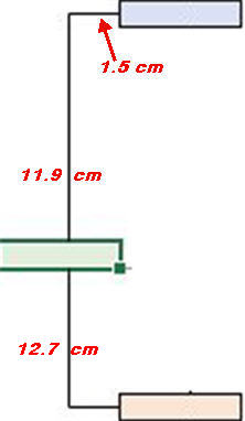
The horizontal lines are 1.5 cm.

Note that the vertical lines are different lengths. The top vertical line is 11.9 cm and the bottom vertical line is 12.7 cm.

This is because the Home Person isn’t perfectly centered. Otherwise, the two cells would fall across the printed page boundary. That would make taping the pages together awkward.

Step 18: Set The Print Area

Because we added a space into column K, Excel will include it in the printout if we don’t take action. That means we would get two extra empty pages.

1. Select the range of cells A1 to J1 to A134 to J134.
2. Go the the Page Layout tab in the top ribbon.
3. Expand the Print Area drop-down.
4. Click “Set Print Area”.

Get Our “Done For You” Bundle

Does this all seem like too much fiddling around? I’ve prepared a bundle of four formatted eight-generation templates.

Two templates have the classic pedigree layout and are designed to print across 4 portrait pages. The other two templates are designed to print across 2 landscape pages.

You can grab them for the price of a good cup of coffee. Download from our Gumroad store.